Schrödinger equation

2007 Schools Wikipedia Selection. Related subjects: General Physics

In physics, the Schrödinger equation, proposed by the Austrian physicist Erwin Schrödinger in 1925, describes the space- and time-dependence of quantum mechanical systems. It is of central importance to the theory of quantum mechanics, playing a role analogous to Newton's second law in classical mechanics.

In the mathematical formulation of quantum mechanics, each system is associated with a complex Hilbert space such that each instantaneous state of the system is described by a unit vector in that space. This state vector encodes the probabilities for the outcomes of all possible measurements applied to the system. As the state of a system generally changes over time, the state vector is a function of time. The Schrödinger equation provides a quantitative description of the rate of change of the state vector.

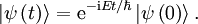
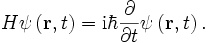
Using Dirac's bra-ket notation, the definition of energy results in the time derivative operator: at time $t$ by $\left|\psi\left(t\right)\right\rangle$ . The Schrödinger equation is

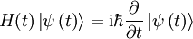
$H(t)\left|\psi\left(t\right)\right\rangle = \mathrm{i}\hbar \frac{\partial}{\partial t} \left| \psi \left(t\right) \right\rangle$

where $i$ is the imaginary unit, $t$ is time, $\partial / \partial t$ is the partial derivative with respect to $t$ , $\hbar$ is the reduced Planck's constant (Planck's constant divided by $2π$ ), $ψ(t)$ is the wave function, and $H\!\left(t\right)$ is the Hamiltonian (a self-adjoint operator acting on the state space).

The Hamiltonian describes the total energy of the system. As with the force occurring in Newton's second law, its exact form is not provided by the Schrödinger equation, and must be independently determined based on the physical properties of the system.

Time-independent Schrödinger equation

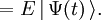
For many real-world problems the energy operator $H$ does not depend on time. Then it can be shown that the time-dependent Schrödinger equation simplifies to the time-independent Schrödinger equation, which—as we will discuss—has the well-known appearance $H Ψ = E Ψ.$

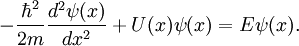
An example of a simple one-dimensional time-independent Schrödinger equation for a particle of mass m, moving in a potential U(x) is:

$-\frac{\hbar^2}{2 m} \frac{d^2 \psi (x)}{dx^2} + U(x) \psi (x) = E \psi (x).$

The analogous 3-dimensional time-independent equation is, :

$\left[-\frac{\hbar^2}{2 m} \nabla^2 + U(r) \right] \psi (r) = E \psi (r).$

For every time-independent Hamiltonian, $H$ , there exists a set of quantum states, $\left|\psi_n\right\rang$ , known as energy eigenstates, and corresponding real numbers $E n$ satisfying the eigenvalue equation,

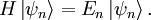
$H \left|\psi_n\right\rang = E_n \left|\psi_n \right\rang.$

Such a state possesses a definite total energy, whose value $E n$ is the eigenvalue of the Hamiltonian. The corresponding eigenvector $\psi_n\,$ is normalizable to unity. This eigenvalue equation is referred to as the time-independent Schrödinger equation. We purposely left out the variable(s) on which the wavefunction $\psi_n\,$ depends. In the first example above it depends on the single variable x and in the second on x, y, and z—the components of the vector r. In both cases the Schrödinger equation has the same appearance, but its Hamilton operator is defined on different function (state, Hilbert) spaces. In the first example the function space consists of functions of one variable and in the second example the function space consists of functions of three variables.

Self-adjoint operators, such as the Hamiltonian, have the property that their eigenvalues are always real numbers, as we would expect, since the energy is a physically observable quantity. Sometimes more than one linearly independent state vector corresponds to the same energy $E n$ . If the maximum number of linearly independent eigenvectors corresponding to $E n$ equals k, we say that the energy level $E n$ is k-fold degenerate. When k=1 the energy level is called non-degenerate.

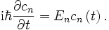
On inserting a solution of the time-independent Schrödinger equation into the full Schrödinger equation, we get

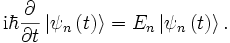
$\mathrm{i} \hbar \frac{\partial}{\partial t} \left| \psi_n \left(t\right) \right\rangle = E_n \left|\psi_n\left(t\right)\right\rang.$

It is relatively easy to solve this equation. One finds that the energy eigenstates (i.e., solutions of the time-independent Schrödinger equation) change as a function of time only trivially, namely, only by a complex phase:

$\left| \psi \left(t\right) \right\rangle = \mathrm{e}^{-\mathrm{i} Et / \hbar} \left|\psi\left(0\right)\right\rang.$

It immediately follows that the probability amplitude,

$\psi(t)^*\psi(t) = \mathrm{e}^{\mathrm{i} Et / \hbar}\mathrm{e}^{-\mathrm{i} Et / \hbar} \psi(0)^*\psi(0) = |\psi(0)|^2,$

is time-independent. Because of a similar cancellation of phase factors in bra and ket, all average (expectation) values of time-independent observables (physical quantities) computed from $\psi(t)\,$ are time-independent.

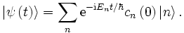
Energy eigenstates are convenient to work with because they form a complete set of states. That is, the eigenvectors $\left\{\left|n\right\rang\right\}$ form a basis for the state space. We introduced here the short-hand notation $|\,n\,\rang = \psi_n$ . Then any state vector that is a solution of the time-dependent Schrödinger equation (with a time-independent $H$ ) $\left|\psi\left(t\right)\right\rang$ can be written as a linear superposition of energy eigenstates:

(The last equation enforces the requirement that $\left|\psi\left(t\right)\right\rang$ , like all state vectors, may be normalized to a unit vector.) Applying the Hamiltonian operator to each side of the first equation, the time-dependent Schrödinger equation in the left-hand side and using the fact that the energy basis vectors are by definition linearly independent, we readily obtain

$\mathrm{i}\hbar \frac{\partial c_n}{\partial t} = E_n c_n\left(t\right).$

Therefore, if we know the decomposition of $\left|\psi\left(t\right)\right\rang$ into the energy basis at time $t = 0$ , its value at any subsequent time is given simply by

$\left|\psi\left(t\right)\right\rang = \sum_n \mathrm{e}^{-\mathrm{i}E_nt/\hbar} c_n\left(0\right) \left|n\right\rang.$

Note that when some values $c_n(0)\,$ are not equal to zero for differing energy values $E_n\,$ , the left-hand side is not an eigenvector of the energy operator $H$ . The left-hand is an eigenvector when the only $c_n(0)\,$ -values not equal to zero belong the same energy, so that $\mathrm{e}^{-\mathrm{i}E_nt/\hbar}$ can be factored out. In many real-world application this is the case and the state vector $\psi(t)\,$ (containing time only in its phase factor) is then a solution of the time-independent Schrödinger equation.

Example

Let $|\,1\,\rangle$ and $|\,2\,\rangle$ be degenerate eigenstates of the time-independent Hamiltonian $H\,$ :

$H\,|\,1\,\rangle = E |\,1\,\rangle \quad \hbox{and} \quad H\,|\,2\,\rangle = E |\,2\,\rangle,$

Suppose at t = 0 a solution $\Psi(t)\,$ of the full Schrödinger equation has the form

$|\,\Psi(t)\,\rangle = \mathrm{e}^{-\mathrm{i}E/\hbar} c_1\left(0\right) |\,1\,\rangle + \mathrm{e}^{-\mathrm{i}E/\hbar} c_2\left(0\right) |\,2\,\rangle,$

then

$H\,|\,\Psi(t)\,\rangle = E \mathrm{e}^{-\mathrm{i}E/\hbar} c_1\left(0\right) |\,1\,\rangle + E\mathrm{e}^{-\mathrm{i}E/\hbar} c_2\left(0\right) |\,2\,\rangle = E\left(\mathrm{e}^{-\mathrm{i}E/\hbar} c_1\left(0\right) |\,1\,\rangle + \mathrm{e}^{-\mathrm{i}E/\hbar} c_2\left(0\right) |\,2\,\rangle\right)$

$= E\,|\,\Psi(t)\,\rangle.$

Conclusion: The wavefunction $\Psi(t)\,$ with the given initial condition (its form at t = 0), remains a solution of the time-independent Schrödinger equation for all times t.

Footnote

^ In fact also an initial condition must be used here. At time zero the wavefunction must be an eigenstate of $H .$

Schrödinger wave equation

The state space of certain quantum systems can be spanned with a position basis. In this situation, the Schrödinger equation may be conveniently reformulated as a partial differential equation for a wavefunction, a complex scalar field that depends on position as well as time. This form of the Schrödinger equation is referred to as the Schrödinger wave equation.

Elements of the position basis are called position eigenstates. We will consider only a single-particle system, for which each position eigenstate may be denoted by $\left|\mathbf{r}\right\rang$ , where the label $\mathbf{r}$ is a real vector. This is to be interpreted as a state in which the particle is localized at position $\mathbf{r}$ . In this case, the state space is the space of all square-integrable complex functions.

The wavefunction

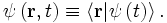
We define the wavefunction as the projection of the state vector $\left|\psi\left(t\right)\right\rang$ onto the position basis:

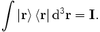
$\psi\left(\mathbf{r}, t\right) \equiv \left\langle \mathbf{r} | \psi\left(t\right) \right\rangle.$

Since the position eigenstates form a basis for the state space, the integral over all projection operators is the identity operator:

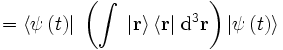
$\int \left|\mathbf{r}\right\rangle \left\langle \mathbf{r} \right| \mathrm{d}^3 \mathbf{r} = \mathbf{I}.$

This statement is called the resolution of the identity. With this, and the fact that kets have unit norm, we can show that

$\left\lang \psi(t) \| \psi(t) \right\rang$	$= \left\lang \psi\left(t\right) \right\| \; \left(\int \; \left\|\mathbf{r}\right\rang \lang\mathbf{r}\| \; \mathrm{d}^3\mathbf{r} \right) \left\|\psi\left(t\right)\right\rang$
	$= \int \; \left\lang\psi\left(t\right)\|\mathbf{r}\right\rang \left\lang\mathbf{r}\|\psi\left(t\right) \right\rang \; \mathrm{d}^3 \mathbf{r}$
	$= \int \; \psi\left(\mathbf{r}, t\right)^* \; \psi\left(\mathbf{r}, t\right) \; \mathrm{d}^3\mathbf{r}$
	$= 1\;$

where $\psi\left(\mathbf{r}, t\right)^*$ denotes the complex conjugate of $\psi\left(\mathbf{r}, t\right)$ . This important result tells us that the absolute square of the wavefunction, integrated over all space, must be equal to 1:

$\int \; \left|\psi\left(\mathbf{r}, t\right)\right|^2 \; \mathrm{d}^3\mathbf{r} = 1.$

We can thus interpret the absolute square of the wavefunction as the probability density for the particle to be found at each point in space. In other words, $\left|\psi\left(\mathbf{r}, t\right)\right|^2 \mathrm{d}^3\mathbf{r}$ is the probability, at time $t$ , of finding the particle in the infinitesimal region of volume $\mathrm{d}^3\mathbf{r}$ surrounding the position $\mathbf{r}$ .

We have previously shown that energy eigenstates vary only by a complex phase as time progresses. Therefore, the absolute square of their wavefunctions do not change with time. Energy eigenstates thus correspond to static probability distributions.

Operators in the position basis

Any operator $A$ acting on the wavefunction is defined in the position basis by

$A \psi\left(\mathbf{r}, t\right) \equiv \left\lang\mathbf{r}| A | \psi\left(t\right) \right\rang.$

The operators A on the two sides of the equation are different things: the one on the right acts on kets, whereas the one on the left acts on scalar fields. It is common to use the same symbols to denote operators acting on kets and their projections onto a basis. Usually, the kind of operator to which one is referring is apparent from the context, but this is a possible source of confusion.

Using the position-basis notation, the Schrödinger equation can be written as

$H \psi\left(\mathbf{r},t\right) = \mathrm{i} \hbar \frac{\partial}{\partial t} \psi\left(\mathbf{r},t\right).$

This form of the Schrödinger equation is the Schrödinger wave equation. It may appear that this is an ordinary differential equation, but in fact the Hamiltonian operator typically includes partial derivatives with respect to the position variable $\mathbf{r}$ . This usually leaves us with a difficult linear partial differential equation to solve.

Non-relativistic Schrödinger wave equation

In non-relativistic quantum mechanics, the Hamiltonian of a particle can be expressed as the sum of two operators, one corresponding to kinetic energy and the other to potential energy. The Hamiltonian of a particle with no electric charge and no spin in this case is:

$H \psi\left(\mathbf{r}, t\right) = \left(T + V\right) \, \psi\left(\mathbf{r}, t\right) = \left[ - \frac{\hbar^2}{2m} \nabla^2 + V\left(\mathbf{r}\right) \right] \psi\left(\mathbf{r}, t\right) = \mathrm{i} \hbar \frac{\partial \psi}{\partial t} \left(\mathbf{r}, t\right)$

where

$T = \frac{p^2}{2m}$ is the kinetic energy operator,

m

is the mass of the particle,

$\mathbf{p} = -\mathrm{i}\hbar\nabla$ is the momentum operator,

$V = V\left(\mathbf{r}\right)$ is the potential energy operator,

V

is a real scalar function of the position operator $\mathbf{r}$ ,

$\nabla$ is the gradient operator, and

$\nabla^2$ is the Laplace operator.

This is a commonly encountered form of the Schrödinger wave equation, though not the most general one. The corresponding time-independent equation is

$\left[ - \frac{\hbar^2}{2m} \nabla^2 + V\left(\mathbf{r}\right) \right] \psi\left(\mathbf{r}\right) = E \psi \left(\mathbf{r}\right).$

The relativistic generalisations of this wave equation are the Dirac equation, Klein-Gordon equation, Proca equation, Maxwell equations etc, depending on spin and mass of the particle. See relativistic wave equations for details.

Probability currents

In order to describe how probability density changes with time, it is acceptable to define probability current or probability flux. The probability flux represents a flowing of probability across space.

For example, consider a Gaussian probability curve centered around $x 0$ with $x 0$ moving at speed $v$ to the right. One may say that the probability is flowing toward right, i.e., there is a probability flux directed to the right.

The probability flux $\mathbf{j}$ is defined as:

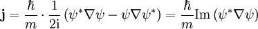
$\mathbf{j} = {\hbar \over m} \cdot {1 \over {2 \mathrm{i}}} \left( \psi ^{*} \nabla \psi - \psi \nabla \psi^{*} \right) = {\hbar \over m} \operatorname{Im} \left( \psi ^{*} \nabla \psi \right)$

and measured in units of (probability)/(area × time) = r⁻²t⁻¹.

The probability flux satisfies a quantum continuity equation, i.e.:

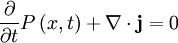
${ \partial \over \partial t} P\left(x,t\right) + \nabla \cdot \mathbf{j} = 0$

where $P\left(x, t\right)$ is the probability density and measured in units of (probability)/(volume) = r⁻³. This equation is the mathematical equivalent of probability conservation law.

It is easy to show that for a plane wave,

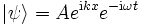
$\left| \psi \right\rang = A e^{ \mathrm{i} k x} e^{ - \mathrm{i} \omega t}$

the probability flux is given by

$j\left(x,t\right) = \left|A\right|^2 {k \hbar \over m}.$

Solutions of the Schrödinger equation

Analytical solutions of the time-independent Schrödinger equation can be obtained for a variety of relatively simple conditions. These solutions provide insight into the nature of quantum phenomena and sometimes provide a reasonable approximation of the behaviour of more complex systems (e.g., in statistical mechanics, molecular vibrations are often approximated as harmonic oscillators). Several of the more common analytical solutions include:

The free particle
The particle in a box
The finite potential well
The Delta function potential
The particle in a ring
The particle in a spherically symmetric potential
The quantum harmonic oscillator
The linear rigid rotor
The symmetric top
The hydrogen atom or hydrogen-like atom
The ring wave guide
The particle in a one-dimensional lattice (periodic potential)

For many systems, however, there is no analytic solution to the Schrödinger equation. In these cases, one must resort to approximate solutions. Some of the common techniques are:

Perturbation theory
The variational principle underpins many approximate methods (like the popular Hartree-Fock method which is the basis of the post Hartree-Fock methods)
Quantum Monte Carlo methods
Density functional theory
The WKB approximation
discrete delta-potential method

Retrieved from " http://en.wikipedia.org/wiki/Schr%C3%B6dinger_equation"

$\left\lang \psi(t) \| \psi(t) \right\rang$	$= \left\lang \psi\left(t\right) \right\| \; \left(\int \; \left\|\mathbf{r}\right\rang \lang\mathbf{r}\| \; \mathrm{d}^3\mathbf{r} \right) \left\|\psi\left(t\right)\right\rang$
	$= \int \; \left\lang\psi\left(t\right)\|\mathbf{r}\right\rang \left\lang\mathbf{r}\|\psi\left(t\right) \right\rang \; \mathrm{d}^3 \mathbf{r}$
	$= \int \; \psi\left(\mathbf{r}, t\right)^* \; \psi\left(\mathbf{r}, t\right) \; \mathrm{d}^3\mathbf{r}$
	$= 1\;$