Ordinary differential equation
2007 Schools Wikipedia Selection. Related subjects: Mathematics
In mathematics, an ordinary differential equation (or ODE) is a relation that contains functions of only one independent variable, and one or more of its derivatives with respect to that variable.
A simple example is Newton's second law of motion, which leads to the differential equation
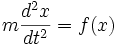 ,
,
for the motion of a particle of mass m. In general, the force f depends upon the position of the particle x, and thus the unknown variable x appears on both sides of the differential equation, as is indicated in the notation f(x).
Ordinary differential equations are to be distinguished from partial differential equations where there are several independent variables involving partial derivatives.
Ordinary differential equations arise in many different contexts including geometry, mechanics, astronomy and population modelling. Many famous mathematicians have studied differential equations and contributed to the field, including Newton, Leibniz, the Bernoullis, Riccati, Clairaut, d'Alembert and Euler.
Much study has been devoted to the solution of ordinary differential equations. In the case where the equation is linear, it can be solved by analytical methods. Unfortunately, most of the interesting differential equations are non-linear and, with a few exceptions, cannot be solved exactly. Approximate solutions are arrived at using computer approximations (see numerical ordinary differential equations).
Definitions
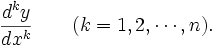
Let y be an unknown function

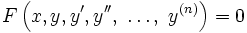
in x with y(i) the i-th derivative of y, then a function

is called an ordinary differential equation (ODE) of order (or degree) n. For vector valued functions

we call F a system of ordinary differential equations of dimension m.
A function y is called a solution of F. A general solution of an nth-order equation is a solution containing n arbitrary variables, corresponding to n constants of integration. A particular solution is derived from the general solution by setting the constants to particular values. A singular solution is a solution that can't be derived from the general solution.
When a differential equation of order n has the form
it is called an implicit differential equation whereas the form
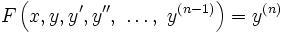
is called an explicit differential equation.
A differential equation not depending on x is called autonomous.
A differential equation is said to be linear if F can be written as a linear combination of the derivatives of y
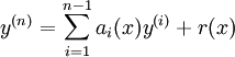
with ai(x) and r(x) continuous functions in x. If r(x)=0 the we call the linear differential equation homogeneous otherwise we call it inhomogeneous.
Examples
Reduction of dimension
Given an explicit ordinary differential equation of order n and dimension 1,
we define a new family of unknown functions
- yn: = y(n − 1).
We can then rewrite the original differential equation as a system of differential equations with order 1 and dimension n.


which can be written concisely in vector notation as
with
Types of ordinary differential equations
Ordinary differential equations which can be categorised by three factors:
- Linear vs. Non-linear
- Homogeneous vs. Inhomogenous
- Constant coefficents versus variable coefficients
Information below provides methods for the solution of these differing ODEs:
Homogeneous linear ODEs with constant coefficients
The first method of solving linear ordinary differential equations with constant coefficients is due to Euler, who realized that solutions have the form ezx, for possibly-complex values of z. Thus to solve
we set y = ezx, leading to

so dividing by ezx gives the nth-order polynomial

In short the terms
of the original differential equation are replaced by zk. Solving the polynomial gives n values of z,  . Plugging those values into
  gives a basis for the solution; any linear combination of these basis functions will satisfy the differential equation.
This equation F(z) = 0, is the "characteristic" equation considered later by Monge and Cauchy.
| Example |
 has the characteristic equation
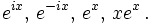
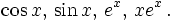
This has zeroes, i, −i, and 1 (multiplicity 2). The solution basis is then
This corresponds to the real-valued solution basis
|
 .
.
If z is a (possibly not real) zero of F(z) of multiplicity m and  then
then  is a solution of the ODE. These functions make up a basis of the ODE's solutions.
If the Ai are real then real-valued solutions are preferable. Since the non-real z values will come in conjugate pairs, so will their corresponding ys; replace each pair with their linear combinations Re(y) and Im(y).
A case that involves complex roots can be solved with the aid of Euler's formula.
- Example: Given
 . The characteristic equation is
 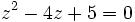 which has zeroes 2+i and 2−i. Thus the solution basis {y1,y2} is
 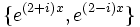 . Now y is a solution iff
  for
for  .
.
Because the coefficients are real,
- we are likely not interested in the complex solutions
- our basis elements are mutual conjugates
The linear combinations
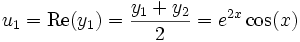 and
and
will give us a real basis in {u1,u2}.
Inhomogeneous linear ODEs with constant coefficients
Suppose instead we face
For later convenience, define the characteristic polynomial

We find the solution basis  as in the homogeneous (f=0) case. We now seek a particular solution yp by the variation of parameters method. Let the coefficients of the linear combination be functions of x:

Using the "operator" notation D = d / dx and a broad-minded use of notation, the ODE in question is P(D)y = f; so

With the constraints


- …

the parameters commute out, with a little "dirt":

But P(D)yj = 0, therefore

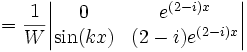
This, with the constraints, gives a linear system in the u'j. This much can always be solved; in fact, combining Cramer's rule with the Wronskian,
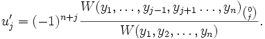
The rest is a matter of integrating u'j.
The particular solution is not unique; 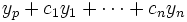 also satisfies the ODE for any set of constants cj.
See also variation of parameters.
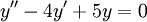
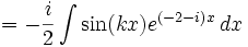
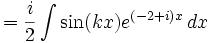
Example: Suppose y'' − 4y' + 5y = sin(kx). We take the solution basis found above {e(2 + i)x,e(2 − i)x}.


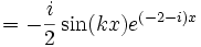

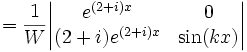
Using the list of integrals of exponential functions

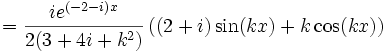

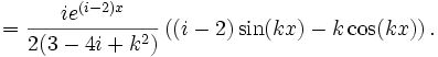
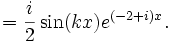
And so


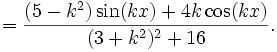
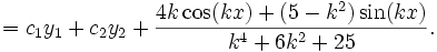
(Notice that u1 and u2 had factors that canceled y1 and y2; that is typical.)
For interest's sake, this ODE has a physical interpretation as a driven damped harmonic oscillator; yp represents the steady state, and c1y1 + c2y2 is the transient.
First-order linear ODEs
| Example |
 with the initial condition
Using the general solution method:
The integration is done from 0 to x, giving:
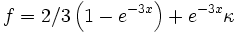
Then we can reduce to:
Assume that kappa is 2 from the initial condition. |
 .
. .
. .
. .
.For a first-order linear ODE, with coefficients that may or may not vary with x:
y'(x) + p(x)y(x) = r(x)
Then,
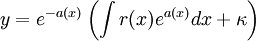
where κ is the constant of integration, and
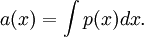
This proof comes from Jean Bernoulli. Let

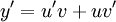
Suppose for some unknown functions u(x) and v(x) that y = uv.
Then
Substituting into the differential equation,
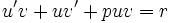
Now, the most important step: Since the differential equation is linear we can split this into two independent equations and write
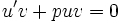

Since v is not zero, the top equation becomes
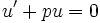
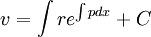
The solution of this is

Substituting into the second equation
Since y = uv, for arbitrary constant C
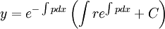
As an illustrative example, consider a first order differential equation with constant coefficients:
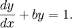
This equation is particularly relevant to first order systems such as RC circuits and mass-damper systems.
In this case, p(x) = b, r(x) = 1.
Hence its solution is

Method of undetermined coefficients
The method of undetermined coefficients (MoUC), is useful in finding solution for yp. Given the ODE P(D)y = f(x), find another differential operator A(D) such that A(D)f(x) = 0. This operator is called the annihilator, and thus the method of undetermined coefficients is also known as the annihilator method. Applying A(D) to both sides of the ODE gives a homogeneous ODE 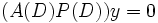 for which we find a solution basis
  as before. Then the original nonhomogeneous ODE is used to construct a system of equations restricting the coefficients of the linear combinations to satisfy the ODE.
Undetermined coefficients is not as general as variation of parameters in the sense that an annihilator does not always exist.
Example: Given y'' − 4y' + 5y = sin(kx), P(D) = D2 − 4D + 5. The simplest annihilator of sin(kx) is A(D) = D2 + k2. The zeros of A(z)P(z) are {2 + i,2 − i,ik, − ik}, so the solution basis of A(D)P(D) is {y1,y2,y3,y4} = {e(2 + i)x,e(2 − i)x,eikx,e − ikx}.
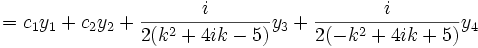
Setting y = c1y1 + c2y2 + c3y3 + c4y4 we find
-
sin(kx) = P(D)y = P(D)(c1y1 + c2y + c3y3 + c4y4) = c1P(D)y1 + c2P(D)y2 + c3P(D)y3 + c4P(D)y4 = 0 + 0 + c3( − k2 − 4ik + 5)y3 + c4( − k2 + 4ik + 5)y4 = c3( − k2 − 4ik + 5)(cos(kx) + isin(kx)) + c4( − k2 + 4ik + 5)(cos(kx) − isin(kx))
giving the system
- i = (k2 + 4ik − 5)c3 + ( − k2 + 4ik + 5)c4
- 0 = (k2 + 4ik − 5)c3 + (k2 − 4ik − 5)c4
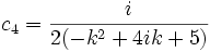
which has solutions
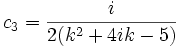 ,
, 
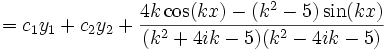
giving the solution set

Method of variation of parameters
As explained above, the general solution to a non-homogeneous, linear differential equation y''(x) + p(x)y'(x) + q(x)y(x) = g(x) can be expressed as the sum of the general solution yh(x) to the corresponding homogenous, linear differential equation y''(x) + p(x)y'(x) + q(x)y(x) = 0 and any one solution yp(x) to y''(x) + p(x)y'(x) + q(x)y(x) = g(x).
Like the method of undetermined coefficients, described above, the method of variation of parameters is a method for finding one solution to y''(x) + p(x)y'(x) + q(x)y(x) = g(x), having already found the general solution to y''(x) + p(x)y'(x) + q(x)y(x) = 0. Unlike the method of undetermined coefficients, which fails except with certain specific forms of g(x), the method of variation of parameters will always work; however, it is significantly more difficult to use.
For a second-order equation, the method of variation of parameters makes use of the following fact:
Fact
Let p(x), q(x), and g(x) be functions, and let y1(x) and y2(x) be solutions to the homogeneous, linear differential equation y''(x) + p(x)y'(x) + q(x)y(x) = 0. Further, let u(x) and v(x) be functions such that u'(x)y1(x) + v'(x)y2(x) = 0 and u'(x)y1'(x) + v'(x)y2'(x) = g(x) for all x, and define yp(x) = u(x)y1(x) + v(x)y2(x). Then yp(x) is a solution to the non-homogeneous, linear differential equation y''(x) + p(x)y'(x) + q(x)y(x) = g(x).
Proof
yp(x) = u(x)y1(x) + v(x)y2(x)
| yp'(x) | = u'(x)y1(x) + u(x)y1'(x) + v'(x)y2(x) + v(x)y2'(x) |
| = 0 + u(x)y1'(x) + v(x)y2'(x) |
| yp''(x) | = u'(x)y1'(x) + u(x)y1''(x) + v'(x)y2'(x) + v(x)y2''(x) |
| = g(x) + u(x)y1''(x) + v(x)y2''(x) |
yp''(x) + p(x)y'p(x) + q(x)yp(x) = g(x) + u(x)y1''(x) + v(x)y2''(x) + p(x)u(x)y1'(x) + p(x)v(x)y2'(x) + q(x)u(x)y1(x) + q(x)v(x)y2(x)
= g(x) + u(x)(y1''(x) + p(x)y1'(x) + q(x)y1(x)) + v(x)(y2''(x) + p(x)y2'(x) + q(x)y2(x)) = g(x) + 0 + 0 = g(x)
Usage
To solve the second-order, non-homogeneous, linear differential equation y''(x) + p(x)y'(x) + q(x)y(x) = g(x) using the method of variation of parameters, use the following steps:
- Find the general solution to the corresponding homogeneous equation y''(x) + p(x)y'(x) + q(x)y(x) = 0. Specifically, find two linearly independent solutions y1(x) and y2(x).
- Since y1(x) and y2(x) are linearly independent solutions, their Wronskian y1(x)y2'(x) − y1'(x)y2(x) is nonzero, so we can compute − (g(x)y2(x)) / (y1(x)y2'(x) − y1'(x)y2(x)) and (g(x)y1(x)) / (y1(x)y2'(x) − y1'(x)y2(x)). If the former is equal to u'(x) and the latter to v'(x), then u and v satisfy the two constraints given above: that u'(x)y1(x) + v'(x)y2(x) = 0 and that u'(x)y1'(x) + v'(x)y2'(x) = g(x). We can tell this after multiplying by the denominator and comparing coefficients.
- Integrate − (g(x)y2(x)) / (y1(x)y2'(x) − y1'(x)y2(x)) and (g(x)y1(x)) / (y1(x)y2'(x) − y1'(x)y2(x)) to obtain u(x) and v(x), respectively. (Note that we only need one choice of u and v, so there is no need for constants of integration.)
- Compute yp(x) = u(x)y1(x) + v(x)y2(x). The function yp is one solution of y''(x) + p(x)y'(x) + q(x)y(x) = g(x).
- The general solution is c1y1(x) + c2y2(x) + yp(x), where c1 and c2 are arbitrary constants.
Higher-order equations
The method of variation of parameters can also be used with higher-order equations. For example, if y1(x), y2(x), and y3(x) are linearly independent solutions to y'''(x) + p(x)y''(x) + q(x)y'(x) + r(x)y(x) = 0, then there exist functions u(x), v(x), and w(x) such that u'(x)y1(x) + v'(x)y2(x) + w'(x)y3(x) = 0, u'(x)y1'(x) + v'(x)y2'(x) + w'(x)y3'(x) = 0, and u'(x)y1''(x) + v'(x)y2''(x) + w'(x)y3''(x) = g(x). Having found such functions (by solving algebraically for u'(x), v'(x), and w'(x), then integrating each), we have yp(x) = u(x)y1(x) + v(x)y2(x) + w(x)y3(x), one solution to the equation y'''(x) + p(x)y''(x) + q(x)y'(x) + r(x)y(x) = g(x).
Example
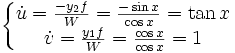
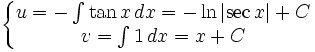
Solve the previous example, y'' + y = secx Recall  . From technique learned from 3.1, LHS has root of
  that yield yc = C1cosx + C2sinx, (so y1 = cosx, y2 = sinx ) and its derivatives
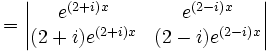
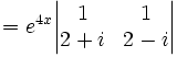
where the Wronskian
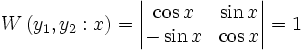
were computed in order to seek solution to its derivatives.
Upon integration,
Computing yp and yG:

Linear ODEs with variable coefficients
A linear ODE of order n with variable coefficients has the general form

Examples
A particular simple example is the Cauchy-Euler equation often used in engineering

Theories of ODEs
Singular solutions
The theory of singular solutions of ordinary and partial differential equations was a subject of research from the time of Leibniz, but only since the middle of the nineteenth century did it receive special attention. A valuable but little-known work on the subject is that of Houtain (1854). Darboux (starting in 1873) was a leader in the theory, and in the geometric interpretation of these solutions he opened a field which was worked by various writers, notably Casorati and Cayley. To the latter is due (1872) the theory of singular solutions of differential equations of the first order as accepted circa 1900.
Reduction to quadratures
The primitive attempt in dealing with differential equations had in view a reduction to quadratures. As it had been the hope of eighteenth-century algebraists to find a method for solving the general equation of the nth degree, so it was the hope of analysts to find a general method for integrating any differential equation. Gauss (1799) showed, however, that the differential equation meets its limitations very soon unless complex numbers are introduced. Hence analysts began to substitute the study of functions, thus opening a new and fertile field. Cauchy was the first to appreciate the importance of this view. Thereafter the real question was to be, not whether a solution is possible by means of known functions or their integrals, but whether a given differential equation suffices for the definition of a function of the independent variable or variables, and if so, what are the characteristic properties of this function.
Fuchsian theory
Two memoirs by Fuchs (Crelle, 1866, 1868), inspired a novel approach, subsequently elaborated by Thomé and Frobenius. Collet was a prominent contributor beginning in 1869, although his method for integrating a non-linear system was communicated to Bertrand in 1868. Clebsch (1873) attacked the theory along lines parallel to those followed in his theory of Abelian integrals. As the latter can be classified according to the properties of the fundamental curve which remains unchanged under a rational transformation, so Clebsch proposed to classify the transcendent functions defined by the differential equations according to the invariant properties of the corresponding surfaces f = 0 under rational one-to-one transformations.
Lie's theory
From 1870 Lie's work put the theory of differential equations on a more satisfactory foundation. He showed that the integration theories of the older mathematicians can, by the introduction of what are now called Lie groups, be referred to a common source; and that ordinary differential equations which admit the same infinitesimal transformations present comparable difficulties of integration. He also emphasized the subject of transformations of contact (Berührungstransformationen).
Sturm-Liouville theory
Sturm-Liouville theory is a general method for resolution of second order linear equations with variable coefficients.