Polar coordinate system

2007 Schools Wikipedia Selection. Related subjects: Mathematics

A polar grid with several angles labeled.

In mathematics, the polar coordinate system is a two-dimensional coordinate system in which points are given by an angle and a distance from a central point known as the pole (equivalent to the origin in the more familiar Cartesian coordinate system). The polar coordinate system is used in many fields, including mathematics, physics, engineering, navigation and robotics. It is especially useful in situations where the relationship between two points is most easily expressed in terms of angles and distance; in the Cartesian coordinate system, such a relationship can only be found through trigonometric formulae. For many types of curves, a polar equation is the simplest means of representation; for some others, it is the only such means.

History

It is known that the Greeks used the concepts of angle and radius. The astronomer Hipparchus (190-120 BC) tabulated a table of chord functions giving the length of the chord for each angle, and there are references to his using polar coordinates in establishing stellar positions. In On Spirals, Archimedes describes his famous spiral, a function whose radius depends on the angle. The Greek work, however, did not extend to a full coordinate system.

There are various accounts of who first introduced polar coordinates as part of a formal coordinate system. The full history of the subject is described in Harvard professor Julian Lowell Coolidge's Origin of Polar Coordinates. Grégoire de Saint-Vincent and Bonaventura Cavalieri independently introduced the concepts at about the same time. Saint-Vincent wrote about them privately in 1625 and published in 1647, while Cavalieri published in 1635 with a corrected version appearing in 1653. Cavalieri first utilized polar coordinates to solve a problem relating to the area within an Archimedean spiral. Blaise Pascal subsequently used polar coordinates to calculate the length of parabolic arcs.

In Method of Fluxions (written 1671, published 1736), Sir Isaac Newton was the first to look upon polar coordinates as a method of locating any point in the plane. Newton examined the transformations between polar coordinates and nine other coordinate systems. In Acta eruditorum (1691), Jacob Bernoulli used a system with a point on a line, called the pole and polar axis respectively. Coordinates were specified by the distance from the pole and the angle from the polar axis. Bernoulli's work extended to finding the radius of curvature of curves expressed in these coordinates.

The actual term polar coordinates has been attributed to Gregorio Fontana and was used by 18th century Italian writers. The term appeared in English in George Peacock's 1816 translation of Lacroix's Differential and Integral Calculus.

Alexis Clairaut and Leonhard Euler are credited with extending the concept of polar coordinates to three dimensions.

Plotting points with polar coordinates

The points (3,60°) and (4,210°)

As with all two-dimensional coordinate systems, there are two polar coordinates: r (the radial coordinate) and θ (the angular coordinate, polar angle, or azimuth angle, sometimes represented as φ or t). The r coordinate represents the radial distance from the pole, and the θ coordinate represents the anticlockwise (counterclockwise) angle from the 0° ray (sometimes called the polar axis), known as the positive x-axis on the Cartesian coordinate plane.

For example, the polar coordinates (3,60°) would be plotted as a point 3 units from the pole on the 60° ray. The coordinates (−3,240°) would also be plotted at this point because a negative radial distance is measured as a positive distance on the opposite ray (240° − 180° = 60°).

One important aspect of the polar coordinate system not present in the Cartesian coordinate system is the ability to express a single point with an infinite number of different coordinates. In general, the point (r, θ) can be represented as (r, θ ± n×360°) or (−r, θ ± (2n + 1)180°), where n is any integer. If the r coordinate of a point is 0, then regardless of the θ coordinate, the point will be located at the pole.

Use of radian measure

Angles in polar notation are generally expressed in either degrees or radians, using the conversion 2π rad = 360°. The choice depends largely on the context. Navigation applications use degree measure, while some physics applications (specifically rotational mechanics) use radian measure, based on the ratio of the radius of the circle to its circumference.

Converting between polar and Cartesian coordinates

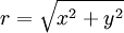
The two polar coordinates r and θ can be converted to Cartesian coordinates by

$x = r \cos \theta \,$

$y = r \sin \theta. \,$

From the above two formulas, r and θ can be defined in terms of x and y:

$r = \sqrt{x^2 + y^2} \,$

$\theta = \begin{cases} \arctan(\frac{y}{x}) & \mbox{if }x>0 \mbox{ and }y\ge0\\ \arctan(\frac{y}{x}) + 2\pi& \mbox{if }x>0 \mbox{ and }y<0\\ \arctan(\frac{y}{x}) + \pi& \mbox{if }x<0\\ \frac{\pi}{2} & \mbox{if }x=0 \mbox{ and }y>0\\ \frac{3\pi}{2} & \mbox{if }x=0 \mbox{ and }y<0 \end{cases}$

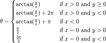
With this formula θ is obtained in [0, 2π), or [0°, 360°).

Polar equations

The equation of a curve expressed in polar coordinates is known as a polar equation, and is usually written with r as a function of θ.

Polar equations may exhibit different forms of symmetry. If r(−θ) = r(θ) then the curve will be symmetrical about the horizontal (0°/180°) ray; if r(π−θ) = r(θ) then it will be symmetric about the vertical (90°/270°); if r(θ−α) = r(θ) then it will be rotationally symmetric α° counterclockwise about the pole.

Circle

A circle with equation r(θ) = 1.

The general equation for any circle with a centre at (r₀, φ) and radius a is

$r^2 - 2 r r_0 \cos(\theta - \varphi) + r_0^2 = a^2$

This can be simplified in various ways, to conform to more specific cases, such as the equation

$r(\theta)=a \,$

for a circle with a centre at the pole and radius a.

Line

Radial lines (those running through the pole) are represented by the equation

$\theta = \varphi \,$ ,

where φ is the angle of elevation of the line; that is, φ = arctan m with m the slope of the line in the Cartesian coordinate system. Any line that does not run through the pole is perpendicular to some radial line. The line that crosses the line θ = φ perpendicularly at the point (r₀, φ) has equation

$r(\theta) = {r_0}\sec(\theta-\varphi) \,$ .

Polar rose

A polar rose with equation r(θ) = 2 sin 4θ.

A polar rose is a famous mathematical curve which looks like a petalled flower, and which can only be expressed as a polar equation. It is given by the equations

$r(\theta) = a \cos k\theta \,$ OR

$r(\theta) = a \sin k\theta \,$

If k is an integer, these equations will produce a k-petalled rose if k is odd, or a 2k-petalled rose if k is even. If k is not an integer, a disc is formed, as the number of petals is also not an integer. Note that with these equations it is impossible to make a rose with 2 more than a multiple of 4 (2, 6, 10, etc.) petals. The variable a represents the length of the petals of the rose.

Archimedean spiral

One arm of an Archimedean spiral with equation r(θ) = θ for 0 < θ < 6π.

The Archimedean spiral is a famous spiral that was discovered by Archimedes, which also can be expressed only as a polar equation. It is represented by the equation:

$r(\theta) = a+b\theta \,$ .

Changing the parameter a will turn the spiral, while b controls the distance between the arms, which is always constant.. The Archimedean spiral has two arms, one for θ > 0 and one for θ < 0. The two arms are smoothly connected at the pole. Taking the mirror image of one arm across the 90°/270° line will yield the other arm. This curve is notable as one of the first known curves where the radius of the function is dependent on the angle, which is the basis of the polar coordinate system.

Conic sections

Ellipse, showing semi-latus rectum

A conic section with one focus on the pole and the other somewhere on the 0° ray (so that the conic's major axis lies along the polar axis) is given by:

$r = {l\over (1 + e \cos \theta)}$

where e is the eccentricity and l is the semi- latus rectum (the perpendicular distance at a focus from the major axis to the curve). If e > 1, this equation defines a hyperbola; if e = 1, it defines a parabola; and if e < 1, it defines an ellipse. The special case e = 0 of the latter results in a circle of radius 1.

Other curves

Because of the circular nature of the polar coordinate system, it is much simpler to describe many curves with an equation in polar rather than Cartesian form. Among the best known of these curves are lemniscates, limaçons, and cardioids.

Complex numbers

Complex numbers, written in rectangular form as a + bi, can also be expressed in polar form in two different ways:

$r(\cos\theta+i\sin\theta) \,$ , abbreviated $r \mbox{ cis } \theta \,$
$r e^{i\theta} \,$

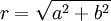
which are equivalent as per Euler's formula. To convert between rectangular and polar complex numbers, the following conversion formulas are used:

$a = r \cos \theta \,$

$b = r \sin \theta \,$

and therefore $r = \sqrt{a^2 + b^2} \,$

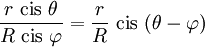
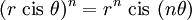
For the operations of multiplication, division, exponentiation, and finding roots of complex numbers, it is much easier to use polar complex numbers than rectangular complex numbers. In abbreviated form:

Multiplication: $(r \mbox{ cis } \theta)(R \mbox{ cis } \varphi) = rR \mbox{ cis } (\theta+\varphi) \,$
Division: $\frac{r \mbox{ cis } \theta}{R \mbox{ cis } \varphi} = \frac{r}{R} \mbox{ cis } (\theta-\varphi) \,$
Exponentiation ( De Moivre's formula): $(r \mbox{ cis } \theta)^n = r^n \mbox{ cis } (n\theta) \,$

Calculus

Calculus can be applied to equations expressed in polar coordinates.

Differential calculus

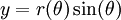
To find the Cartesian slope of the tangent line to a polar curve r(θ) at any given point, the curve is first expressed as a system of parametric equations.

$x=r(\theta)\cos(\theta) \,$

$y=r(\theta)\sin(\theta) \,$

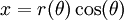
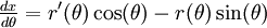
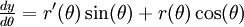
Differentiating both equations with respect to θ yields

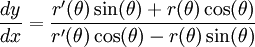
$\tfrac{dx}{d\theta}=r'(\theta)\cos(\theta)-r(\theta)\sin(\theta) \,$

$\tfrac{dy}{d\theta}=r'(\theta)\sin(\theta)+r(\theta)\cos(\theta) \,$

Dividing the second equation by the first yields the Cartesian slope of the tangent line to the curve at the point (r, r(θ)):

$\frac{dy}{dx}=\frac{r'(\theta)\sin(\theta)+r(\theta)\cos(\theta)}{r'(\theta)\cos(\theta)-r(\theta)\sin(\theta)}$

Integral calculus

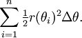
To find the area under a curve r(θ) on a closed interval [a, b], where 0 < b − a < 2π, the curve is first expressed as a Riemann sum. First the interval [a, b] is divided into n subintervals, where n is an arbitrary positive integer. Thus Δθ, the length of each subinterval, is equal to b − a (the total length of the interval), divided by n, the number of subintervals. For each subinterval i = 1, 2, …, n, let θ_i be the midpoint of the subinterval, and construct a sector with the centre at the pole, radius r(θ_i), and central angle Δθ. The area of each constructed sector is therefore equal to $\tfrac12r(\theta_i)^2\Delta\theta$ . Hence, the total area of all of the sectors is

$\sum_{i=1}^n \tfrac12r(\theta_i)^2\Delta\theta.$

As the number of subintervals n is increased, the approximation of the area continues to improve. Thus, the area under the curve r(θ) on [a, b] can be defined as

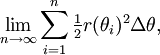
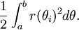
$\lim_{n \to \infty} \sum_{i=1}^n \tfrac12r(\theta_i)^2\Delta\theta,$

the Riemann sum for the integral

$\frac12\int_a^b r(\theta_i)^2 d\theta.$

Vector calculus

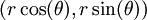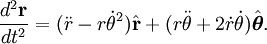
Vector calculus can also be applied to polar coordinates. Let $\mathbf{r}$ be the position vector $(r\cos(\theta),r\sin(\theta))\,$ , with r and $θ$ depending on time t, $\hat{\mathbf{r}}$ be a unit vector in the direction $\mathbf{r}$ and $\hat{\boldsymbol\theta}$ be a unit vector at right angles to $\mathbf{r}$ . The first and second derivatives of position are

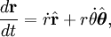$\frac{d\mathbf{r}}{dt} = \dot r\hat{\mathbf{r}} + r\dot\theta\hat{\boldsymbol\theta},$ .

$\frac{d^2\mathbf{r}}{dt^2} = (\ddot r - r\dot\theta^2)\hat{\mathbf{r}} + (r\ddot\theta + 2\dot r \dot\theta)\hat{\boldsymbol\theta}.$

Let $\mathbf{A}$ be the area swept out by a line joining the focus to a point on the curve. In the limit $d\mathbf{A}$ is half the area of the parallelogram formed by $\mathbf{r}$ and $d\mathbf{r}$ ,

$dA = \begin{matrix}\frac{1}{2}\end{matrix} |\mathbf{r} \times d\mathbf{r}|$ ,

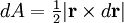and the total area will be the integral of $d\mathbf{A}$ with respect to time.

Three dimensions

The polar coordinate system is extended into three dimensions with two different coordinate systems, the cylindrical and spherical coordinate systems, both of which include the two-dimensional polar coordinates as a subset.

Cylindrical coordinates

2 points plotted with cylindrical coordinates

The cylindrical coordinate system is a coordinate system that essentially extends the two-dimensional polar coordinate system by adding a third coordinate measuring the height of a point above the plane, similar to the way in which the Cartesian coordinate system is extended into three dimensions. The third coordinate is usually denoted h, making the three cylindrical coordinates (r, θ, h).

The three cylindrical coordinates can be converted to Cartesian coordinates by

${x}={r} \,\cos\theta$

${y}={r} \, \sin\theta$

${z}={h} \,$

Spherical coordinates

A point plotted using spherical coordinates

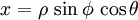
Polar coordinates can also be extended into three dimensions using the coordinates (ρ, φ, θ), where ρ is the distance from the pole, φ is the angle from the z-axis (called the colatitude or zenith and measured from 0 to 180°) and θ is the angle from the x-axis (as in the polar coordinates). This coordinate system, called the spherical coordinate system, is similar to the latitude and longitude system used for Earth, with the latitude being the complement of φ, determined by δ = 90° − φ, and the longitude being measured by l = θ − 180°.

The three spherical coordinates are converted to Cartesian coordinates by

$x =\rho \, \sin\phi \, \cos\theta$

$y =\rho \, \sin\phi \, \sin\theta$

$z =\rho \, \cos\phi$

Applications

Robotics

Many robots capable of movement use the polar coordinate system (or a slightly modified version of it) for navigation. This is very convenient for artificial intelligence, as the centre of the coordinate system (the pole) is always placed at the robot's present location. Therefore, the robot need not calculate where it is within the coordinate system at any given time; all it needs to determine is in which direction and how far to move. If robots were to navigate using the Cartesian coordinate system, distance and angles required for movement would have to be calculated using algebra and trigonometry. In the polar coordinate system, a robot simply needs to be told how far to move, and in what direction (given as an angle), and the robot knows exactly where to go.

Aviation

In the air, aircraft use a slightly modified version of the polar coordinate system for navigation. In this coordinate system, the 0° ray (generally called heading 360) is vertical, and the angles continue in a clockwise, rather than a counterclockwise, direction. Heading 360 corresponds to magnetic north, while headings 90, 180, and 270 correspond to magnetic east, south, and west, respectively. Thus, an aircraft traveling 5 nautical miles due east will be traveling 5 units at heading 90 (read niner-zero by air traffic control).

Archimedean spiral

The Archimedean spiral has many real-world applications. Scroll compressors, made from two interleaved Archimedean spirals of the same size, are used for compressing liquids and gases. The grooves of very early gramophone records form an Archimedean spiral, making the grooves evenly spaced and maximizing the amount of music that could be fit onto the record (although this was later changed to allow better sound quality). Archimedean spirals are also used in DLP projection systems to minimize the "Rainbow Effect", making it look as if multiple colors are displayed at the same time, when in reality red, green, and blue are being cycled extremely fast.

Retrieved from " http://en.wikipedia.org/wiki/Polar_coordinate_system"